Hedge Fund Performance – Is Sharpe Ratio an Ideal Measure?

A metric prominently used in the Hedge fund industry is the Sharpe ratio. The Sharpe ratio measures the amount of return adjusted for each level of risk taken. It is calculated by subtracting the risk-free rate from annualized returns and dividing the result by the standard deviation of the returns.

The mathematical representation is as below:

Sharpe Ratio:

S(x) = (rx – Rf )/StdDev(x)

where,

• x is the investment
• rx is the average rate of return of x
• Rf is the best available rate of return of a risk-free security (i.e. T-bills)
• StdDev(x) is the standard deviation of rx

The Sharpe ratio helps make the performance of one fund comparable to another fund by adjusting for risk where risk is represented by the returns standard deviation. It is useful in determining if holding a riskier asset is worth the added volatility and return. If not, then it’s probably better to not invest in that asset.

Let’s look at an example to understand this well. If Fund A generates a return of 13% while Fund B generates a return of 15%, then it seems that Fund B is the better performer. However, it is possible that Fund B probably took on much more risk to generate the higher return, in which case the added return is not on account of better skills but simply a compensation for increased risk of the Fund.

Continuing on with the previous example, suppose that Fund A has a standard deviation of 8% while Fund B has a standard deviation of 11%, and the risk free rate is 3%. Based on this information, the Sharpe ratio for Fund A is 1.25 while for Fund B is 1.09. Therefore, we can say that the Fund A actually performed better on a risk-adjusted basis.

Despite the popularity of the Sharpe ratio in the portfolio management industry, the ratio is not without its issues and limitations.

Imposes a Normality Assumption on Asset Returns
One of the reasons that Sharpe ratio does not capture the real world is that it relies on standard deviation, which is based on the normal distribution curve (assumes returns are normally distributed). Deviation from normality may generate a biased assessment of performance when using the Sharpe ratio. If returns from hedge funds were normally distributed, then we would expect
to see a concentration of returns within one standard deviation of the mean. This is usually far from what is actually observed.

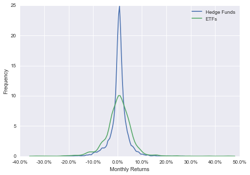
We studied 172 Hedge Funds and 48 ETFs on RADiENT and compared their return distributions for the period 2012 to 2015. From the below distribution curve it can be observed that the deviation from normality is much more in Hedge Funds compared to ETFs.

Penalizes Both Upside and Downside Volatility
Another weakness of the Sharpe ratio is the way it treats all volatility the same. High outlier returns can have the effect of increasing the value of the denominator (standard deviation) more than the value of the numerator, thereby lowering the value of the ratio.

To consider an extreme example, assume two portfolios as shown below:
1. 50% chance of 7% return, 50% chance of 13% return
2. 50% chance of 7% return, 50% chance of 25% return

The Sharpe ratios for these portfolios will be:

Portfolio 2 is clearly better than Portfolio 1 but its Sharpe ratio is lower. A suggested improvement is considering only the negative semi-standard deviation for the denominator, a measure known as Sortino ratio.

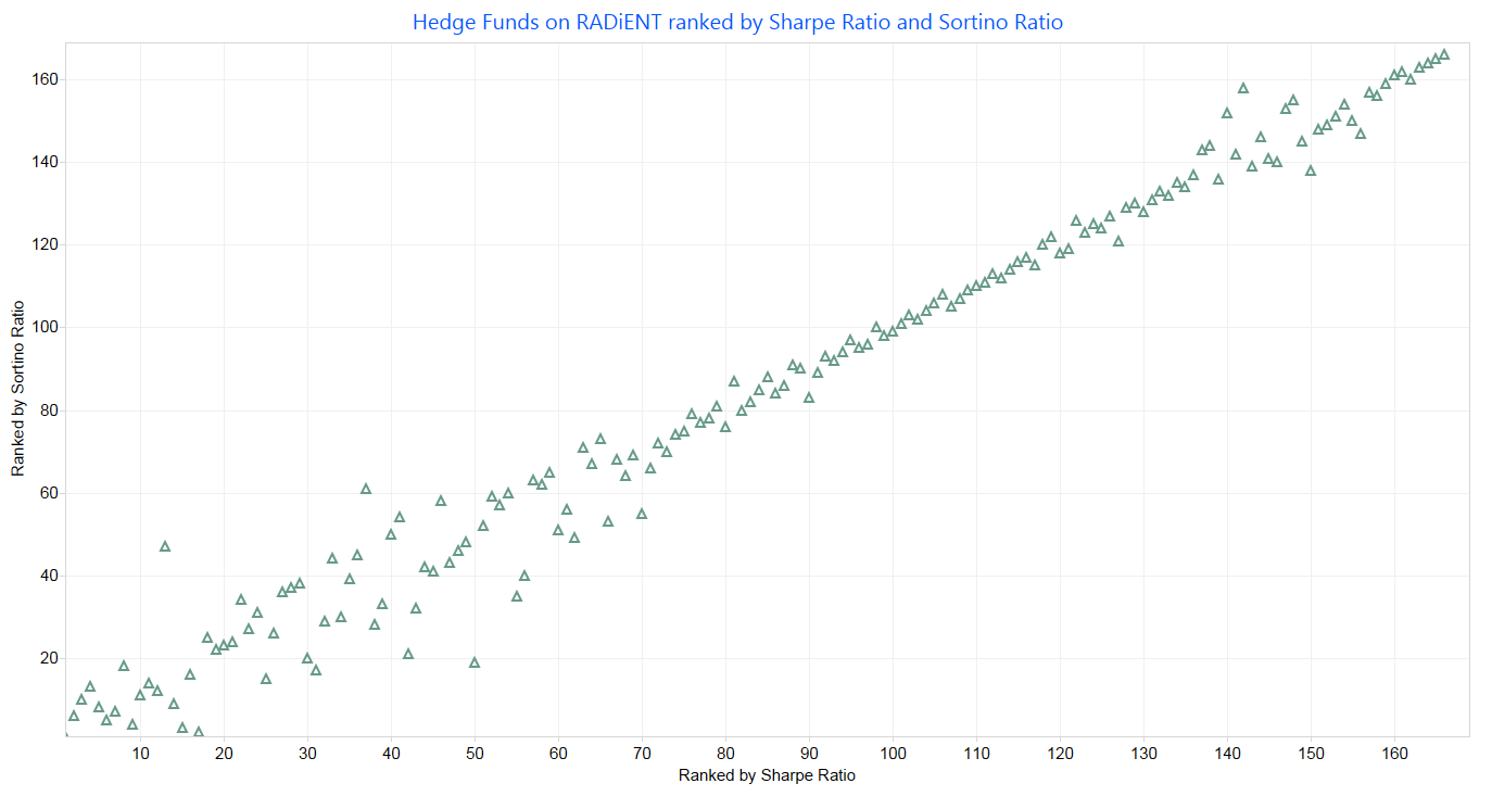
Ranking of funds based on Sharpe ratio and Sortino ratio can lead to different results since while Sharpe ratio considers both upside and downside volatility of returns as a measure of risk, the Sortino ratio considers only the downside deviation of returns. To study this, we compared all Hedge Funds on RADiENT and ranked them individually by their calculated Sharpe ratio and Sortino ratio (as shown in figure below). As observed, both measures provide different ranking of funds.

Sharpe Ratio Differs When Calculated using Data of Different Time Granularity
Lengthening the measurement interval will not alter returns, but will generally, for most asset classes, lower the standard deviation and upwardly bias the Sharpe ratio.

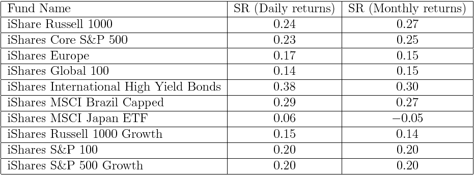
Below is an extract from our study of Exchange Traded Funds (ETFs) on RADiENT. We calculated the annualized Sharpe ratio of ETFs using their daily and monthly returns and compared the two to highlight the divergences in observed Sharpe ratios. We did not use Hedge Funds for the purpose of this study as Hedge fund returns are reported on monthly basis.

Difficulty in Comparing Sharpe Ratio
Because Sharpe ratio is a dimensionless ratio, it is difficult to interpret Sharpe ratio of different investments. It is important to note that the it is an ordinal measure meaning that the order matters, but not the difference between values. For example, a fund with a Sharpe ratio of 1.3 is better compared to a fund with Sharpe ratio of 0.4, but the distance between the two Sharpe
ratios does not provide any insight into how better one fund is compared to the other.

Ignores Serial Correlation in Returns
Sharpe ratio ignores the serial correlation between hedge fund returns. If serial correlation is present in month-to-month returns, the same can result in overstating the Sharpe ratio. This is because serial correlation leads to smoothing of returns. According to Andrew Lo in `The Statistics of Sharpe Ratios’, serial correlation has dramatic effects on the annual Sharpe ratios of hedge funds, inflating it by more than 65 percent in some cases, and understating it in the case of negatively serially correlated returns.

Summary
Despite its flaws, the Sharpe ratio is still the predominant measure of risk-adjusted performance. This can possibly be attributed to its ease of use and the fact that it relies on the investments own numbers than on external index benchmarks used in other measures such as alpha and beta.

There are various other risk-adjusted performance measures which attempt to overcome the limitations of Sharpe ratio such as Modified Sharpe Ratio (MSR), Sortino ratio, etc. However, no measure is without its own limitations. It is therefore important to use the Sharpe ratio in conjunction with other measures to arrive at the complete picture.

 

---

Shivam Singhal is a Business Analyst in the India Innovation Lab at Risk Advisors Inc. in Mumbai. He focuses on client projects related to investor reporting and performance measurement, and on defining similar metrics for our in-house fund analytics platform.

Previously, he worked in the Risk Management department under the Capital Markets division at Kotak Mahindra Group, a banking and financial services firm in India. He was responsible for the preparation of various risk related reports, ensuring compliance with company risk policy. Additionally, he was actively involved in system analysis for new product developments, and identifying areas for efficiency improvements in existing processes.

Shivam is a Chartered Accountant and is currently a CFA Level 3 candidate.